For my end of term project in using the program Microsoft
Excel, I had to use my knowledge acquired on the functions of various formulas
that can be used to create a spreadsheet that served a real life purpose. I
decided to incorporate a topic of personal interest, books (since I love
reading) into my final product.
The primary focus for my Excel spreadsheet was based on a
bookstore, and I developed this focus into the finances in a bookstore so that
it was applicable for the formulas used in Microsoft Excel. I decided that my
spreadsheet would be a Monthly Sales report for a local bookstore based on some
basic data that I typed in.
To start off with, my first step was to create a checklist
for all the features, numbers and formulas I wanted to include in my
spreadsheet as a kind of plan for when I created it using Excel, along with a
few simple guidelines for the business to follow when handling things such as
stock, etc. to serve as rules for the data to mimic:

Next, I created the actual thing on Excel using formulas
that we learnt about in classs, including a few such as
·
=IF([condition], “ “, “ “): the If formula is
used to format the cell to display specific text under conditions that you have
set in reference to another part of the spreadsheet e.g. I used it in places
like the Inventory table, where I formatted the cells to display “STOCK RUNNING
LOW” if the numbers dropped below 300 pieces in tock, listening to one
specification I had set in the beginning
·
=SUM([cell]:[cell]): the SUM formula is used to find
the total added value of two or more cells in the spreadsheet, e.g. I used it
in situations where I had to find the total cost of certain numbers such as
expenditures and overall monthly income for the bookstore
·
Some formulas include operations as simple as
multiplication, division and subtraction by using the *, /, and – signs
respectively in between cell references in situations such as finding the stock
at the end of the month by using subtraction to calculate the difference
between the stock at the beginning and the amount of pieces sold when doing
inventory for the bookstore
·
When using formulas such as the previous
examples given, sometimes you want a whole column to use the data value in a
fixed cell at one point during the equation, for example, I used it to
calculate things such as shipping costs or tax revenue generated by using the
percentage value written in one specific cell – this is called a relative cell reference, where you insert
a ‘$’ symbol before and after the column of the cell that you’re referencing is
in within the formula in order to fix the value in place when continuing said
formula throughout multiple cells.
When creating my product, I also utilised a new, unfamiliar
feature of Microsoft Excel that we had not learnt about in class after doing my
own research to find out its function to highlight certain features of my
spreadsheet; it is called Conditional Formatting. Conditional formatting is
something that allows you to create and set rules and use formatting effects to
emphasize specific data in selected cells of my Excel spreadsheet; a few
formatting effects include gradients, highlights, colour fills, text colours, icons,
and data bars to cells that show specific values, text, content, or even the
Top/Bottom 10 values and percentages in the area that you have chosen in your
spreadsheet:

I wanted to use it in order to turn the text in the Stock
Status column of my Inventory table a bright red if it indicated that the stock
was running low, as a sort of caution or warning for the users of the
spreadsheet to re-stock.
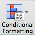
1.
The first step was to select the Conditional
Formatting tool in the ‘Home’ bar of your Excel window:
2.
Next, you click on “New Rule…” to add/set a rule
for the selected cells of your spreadsheet to follow:

3.
Select the style of formatting effects that you
want to apply (I chose the ‘Classic’ option):

4.
Select the nature of the cells you want to
format, e.g. ‘cells that contain…’; I chose this option as it allows me
more freedom over what type of cell I want to control:

5.
Select what you want the type of cell that is
altered to contain, e.g. number values, percentages, specific text – I chose
the latter,, and then in then typed in “STOCK RUNNING LOW” in the blank,
setting the rule to alter only cells that displayed the chosen words:
6.
Choose what kind of effect you wish to apply to
said cells; there is a small preview bar next to it that lets you view the
effect you desire before it is applied to your document:

7.
Press ‘OK’, and your rule is set!

Overall, I am very happy with how I’ve applied my previously
acquired and newly researched knowledge of functions in the program Microsoft
Excel to create my own spreadsheet that showcases my skills in working with
said software, and I am content with the way that my finished product shows an
original real life application of it, especially since a lot of the things I
explored and learnt were quite new to me.
This whole unit has been interesting as this aspect of Excel was
unfamiliar to me, and I feel that I can easily use this in some of my other
subjects too, now, such as Maths, Science and Food Technology for things like
calculating and displaying results of investigations, experiments, and reviews
on expenditures. I personally feel that the topic successfully incorporates the
IB MYP Global Context of ‘Scientific and Technical Innovation’ very well to
teach us transdisciplinary skills, and was on the whole a very interesting one.
No comments:
Post a Comment